Kinematics

Kinematics is the creation of a mathematical model of an object's motion.  An object is moving when its position changes over time. Therefore, motion can be modelled as a function of position with respect to time.  So, the first step in modelling an object's motion is to model an object's position.  This can be achieved by selecting a coordinate system with sufficient dimensions \(n\).  Typically, in classical mechanics, \(n = 3\) for most real-world scenarios, as we live in a (perceived) three-dimensional world. But we may also use \(n = 2\) when we only care about motion restricted to a plane. Any point within such a system can be described using a sequence of \(n\) values. These values form the components or coordinates of the point. The point's position may then be modelled as an \(n\)-dimensional vector, known as the position vector, whose values are the coordinates of the point. 

Selection of a coordinate system requires four considerations:

• Selecting the type of coordinate system (Cartesian, polar, etc.)
• Selecting a reference point (the origin) from which all other positions are relative.
• Defining the orientation of the axes of the coordinate system.
• Selecting units of measurement for each component of the coordinates.

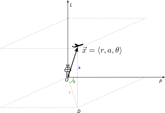
Consider the example of an air traffic control system which must keep track of the position of aircraft within its airspace.  Figure 1.1 demonstrates one way of choosing a coordinate system for this situation.

In this scenario, a 3-dimensional cylindrical coordinate system has been chosen.  Such a system requires specifying an origin at which two axes — the polar and longitudinal axes — intersect.  Let the control tower be the origin \(O\), and let the polar axis \(P\) be the line that is drawn from the control tower due north.  The longitudinal axis \(L\) will be the line perpendicular to the Earth's surface, emerging from \(O\).  Any aircraft position may now be represented with a position vector \(\vec{x} = \langle r, a, \theta \rangle \). The length \(r\) represents the radial distance from the control tower to the point on the ground directly underneath the aircraft, designated by the point \(D\).  The length \(a\) represents the altitude or height of the aircraft above the ground. Finally, the angle \(\theta\) is the clockwise-positive angle subtended between the line \(OD\) and the axis \(A\). We will assert the lengths \(a\) and \(r\) be measured in meters, and \(\theta\) to be measured in degrees.  If the aircraft in the diagram is 6km northwest of the control tower at a height of 5000 meters, the position vector \(\vec{x}\), represented by the black arrow, will have the value \(\langle 6000\text{m}, 5000\text{m}, 45° \rangle \).

 

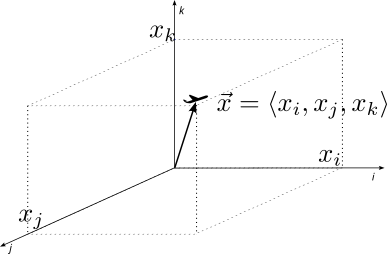
Within most texts on classical mechanics, and this one being no exception, a Cartesian coordinate system is more common for modelling kinematics scenarios.  A Cartesian coordinate system (Figure 1.2) defines three orthogonal axes \(i\), \(j\) and \(k\), which all intersect at the origin.  A point \(P\) in this space can be represented by the position vector \(\vec{P} = \langle x_i, x_j, x_k \rangle\), where \(x_i\), \(x_j\) and \(x_k\) represent the projections of the point \(P\) on the \(i\), \(j\) and \(k\) axes, respectively.

With the choice of a coordinate system, we are now ready to model motion mathematically.  We define the vector function \(\vec{x}(t)\) of some object to be the function that yields the position vector for the object at some time \(t\).  As an example, consider the Cartesian position function \(\vec{x}(t) = a \cos(t)\uveci + a \sin(t)\uvecj + t\uvec{k}, t \ge 0\).  The terms \(\uveci, \uvecj, \text{and } \uvec{k}\) represent the unit vectors for the \(i, j \text{ and } k\) axes respectively. This function models an object whose position is \(\langle 1, 0, 0\rangle\) at \(t = 0\).  As \(t\) increases, the object travels a spiral path upwards and anti-clockwise around the \(k\) axis, with the radius of the spiral being \(a\) units.  The spiral performs one complete revolution every \(2 \pi \) units of time, and grows in height by one unit for each unit of time.  

 

Velocity

Velocity is defined as the rate of change of an object's position.  Velocity is a vector quantity whose magnitude is sometimes known as speed.  Recall from mathematics that the average rate of change of some function \(f(x)\) between two values \(x_1\) and \(x_2\) is defined as \(\frac{f(x_2) - f(x_1)}{x_2 - x_1}\).  We therefore define the average velocity of an object as:

\[{\vec{v}}_{avg} = \frac{\Delta \vec{x}}{\Delta t} = \frac{\vec{x_2} - \vec{x_1}}{t_2 - t_1}\]

where \(\vec{x_1}\) and \(\vec{x_2}\) are the position vectors of the object at times \(t_1\) and \(t_2\) respectively.  For example, if an object has the position vectors \(\vec{x_1} = -3\uveci + \uvecj + 6\uvec{k}\) at time \(t_1 = 5\), and \(\vec{x_2} = 2\uveci - \uvecj - \uvec{k}\) at time \(t_2 = 10\), then we can calculate the average velocity between these times.  That is, \({\vec{v}}_{avg} = \frac{\vec{x_2} - \vec{x_1}}{t_2 - t_1}\) \(= \frac{(2\uveci - \uvecj - \uvec{k}) - (-3\uveci + \uvecj + 6\uvec{k})}{10 - 5}\) \(= \frac{5\uveci - 2\uvecj -7\uvec{k}}{5}\) \(= \uveci - \frac{2}{5}\uvecj - \frac{7}{5}\uvec{k}\).

If an object's position function \(\vec{x}(t)\) can be represented as a differentiable algebraic expression, we can derive an instantaneous velocity function \(\vec{v}(t)\) which allows us to calculate the instantaneous velocity of the object at any time \(t\).  From calculus, we know that the derivative function of some function \(f(x)\), denoted as\(\frac{\text{d}f}{\text{d}x}\), is a function that yields the instantaneous rate of change of \(f(x)\) for any \(x\).  So, the instantaneous velocity function is given by:

\[\vec{v}(t) = \frac{\text{d}\vec{x}}{\text{d}t}\]

When \(\vec{v}(t) = \vec{0}\), the object is not moving (it is at rest).  As an example, let the position function for some object be \(\vec{x}(t) = 4t^2\uveci - t^3\uvecj - \uvec{k}\).  Then, the velocity function \(\vec{v}(t) = \frac{\text{d}\vec{x}}{\text{d}t} = 8t\uveci - 3t^2\uvecj \).

Acceleration

Acceleration is defined as the rate of change of an object's velocity.  Just like velocity, acceleration is a vector quantity.  Using the same reasoning outlined in the preceding section, it should be easy to conclude that the average acceleration \({\vec{a}}_{avg}\) of an object is defined as:

\[{\vec{a}}_{avg} = \frac{\Delta \vec{v}}{\Delta t} = \frac{\vec{v_2} - \vec{v_1}}{t_2 - t_1}\]

where \(\vec{v_1}\) and \(\vec{v_2}\) are the velocity vectors of the object at times \(t_1\) and \(t_2\) respectively.  For example, if an object has the velocity vectors \(\vec{v_1} = 2\uveci - \uvecj - 6\uvec{k}\) at time \(t_1 = 4\), and \(\vec{v_2} = 10\uveci + \uvecj\) at time \(t_2 = 12\), then we can calculate the average acceleration between these times.  That is, \({\vec{a}}_{avg} = \frac{\vec{v_2} - \vec{v_1}}{t_2 - t_1}\) \(= \frac{(10\uveci + \uvecj) - (2\uveci - \uvecj - 6\uvec{k})}{12 - 4}\) \(= \frac{8\uveci + 2\uvecj + 6\uvec{k}}{8}\) \(= \uveci + \frac{1}{4}\uvecj + \frac{3}{4}\uvec{k}\).

An object's acceleration function \(\vec{a}(t)\) is simply the derivative of the velocity function \(\vec{v}(t)\):

\[\vec{a}(t) = \frac{\text{d}\vec{v}}{\text{d}t} = \frac{\text{d}^2\vec{x}}{\text{d}t^2}\]

When \(\vec{a}(t) = \vec{0}\), the object is moving at a constant velocity.  The acceleration function of the object in the above example would be \(\vec{a}(t) = 8\uveci - 6t\uvecj\).

Deriving the equations of motion

We have shown how to find the functions for velocity and acceleration of an object, given the position function of the object, by differentiation. We can also do the reverse, and derive the functions for velocity and displacement from the acceleration function via integration. However, we require some initial conditions to be known; specifically, the initial velocity and initial displacement (velocity and displacement at \(t = 0\)).  Given the acceleration function \(\vec{a}(t)\) of an object, and its velocity at \(t = 0\) (\(v_0\)), the velocity function of the object is:

\[\vec{v}(t) = \int \vec{a}(t) \text{ d}t\]

where the constant of integration will be replaced with \(v_0\).  We can then integrate the velocity function, and knowing the displacement of the object at \(t = 0\) (\(x_0\)), the displacement function will be:

\[\vec{x}(t) = \int \vec{v}(t) \text{ d}t\]

where the constant of integration will be replaced with \(x_0\).

Equations of motion: constant acceleration

An important scenario in classical mechanics is that of an object experiencing a constant acceleration.  That is, \(a(t) = \vec{A}\), where \(\vec{A}\) is a vector constant.  The canonical example is an object in free fall close to the Earth's surface.  Projectile motion is another example which has practical aeronautical and military applications.  If we know the initial velocity \(\vec{v}_0\) of such an object, then according to Kin 1.1, we get:

\[\vec{v}(t) = \vec{v}_0 + \vec{A}t \]

Integrating once again to get the displacement function, we get:

\[\vec{x}(t) = \vec{x}_0 + \vec{v}_0t + \frac{1}{2}\vec{A}t^2 \]